Additional methods

This notebooks provides an overview of built-in clustering performance evaluation, ways of accessing individual labels resulting from clustering and saving the object to disk.

Clustering performance evaluation

Clustergam includes handy wrappers around a selection of clustering performance metrics offered by scikit-learn. Data which were originally computed on GPU are converted to numpy on the fly.

Let’s load the data and fit clustergram on Palmer penguins dataset. See the Introduction for its overview.

import seaborn
from sklearn.preprocessing import scale
from clustergram import Clustergram

seaborn.set(style='whitegrid')

df = seaborn.load_dataset('penguins')
data = scale(df.drop(columns=['species', 'island', 'sex']).dropna())

cgram = Clustergram(range(1, 12), n_init=10, verbose=False)
cgram.fit(data)

Clustergram(k_range=range(1, 12), backend='sklearn', method='kmeans', kwargs={'n_init': 10})

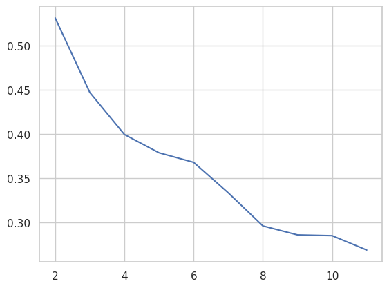
Silhouette score

Compute the mean Silhouette Coefficient of all samples. See scikit-learn documentation for details.

cgram.silhouette_score()

2     0.531540
3     0.447219
4     0.399584
5     0.378848
6     0.368051
7     0.333516
8     0.296052
9     0.285892
10    0.285010
11    0.268741
Name: silhouette_score, dtype: float64

Once computed, resulting Series is available as cgram.silhouette_. Calling the original method will recompute the score.

cgram.silhouette_.plot();

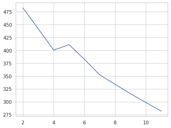
Calinski and Harabasz score

Compute the Calinski and Harabasz score, also known as the Variance Ratio Criterion. See scikit-learn documentation for details.

cgram.calinski_harabasz_score()

2     482.191469
3     441.677075
4     400.410025
5     410.999843
6     382.480417
7     352.276772
8     334.044560
9     315.710033
10    298.716086
11    281.887865
Name: calinski_harabasz_score, dtype: float64

Once computed, resulting Series is available as cgram.calinski_harabasz_. Calling the original method will recompute the score.

cgram.calinski_harabasz_.plot();

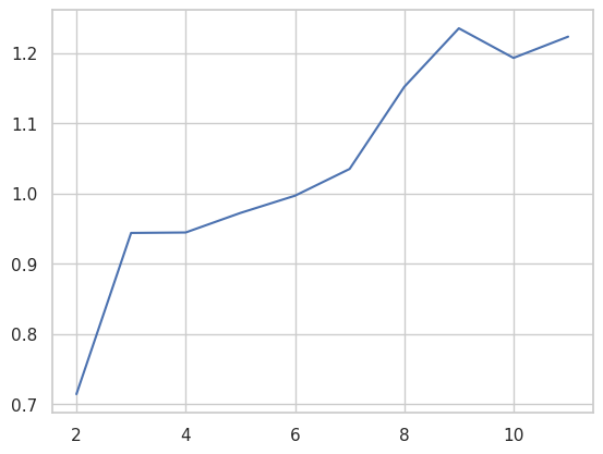
Davies-Bouldin score

Compute the Davies-Bouldin score. See scikit-learn documentation for details.

cgram.davies_bouldin_score()

2     0.714064
3     0.943553
4     0.944215
5     0.971992
6     0.996543
7     1.034658
8     1.151462
9     1.234888
10    1.192744
11    1.222995
Name: davies_bouldin_score, dtype: float64

Once computed, resulting Series is available as cgram.davies_bouldin_. Calling the original method will recompute the score.

cgram.davies_bouldin_.plot();

Acessing labels

Clustergram stores resulting labels for each of the tested options, which can be accessed as:

cgram.labels_

	1	2	3	4	5	6	7	8	9	10	11
0	0	0	2	2	4	1	1	3	5	8	3
1	0	0	2	2	4	1	1	0	5	8	3
2	0	0	2	2	4	1	1	0	5	0	4
3	0	0	2	2	4	1	1	3	4	0	8
4	0	0	2	2	1	4	2	3	4	6	8
...	...	...	...	...	...	...	...	...	...	...	...
337	0	1	1	0	0	0	3	7	0	7	2
338	0	1	1	0	0	0	3	7	0	7	2
339	0	1	1	3	3	3	0	5	3	4	0
340	0	1	1	0	0	0	6	1	8	1	7
341	0	1	1	3	3	3	6	1	8	1	7

342 rows × 11 columns

Saving clustergram

If you want to save your computed clustergram.Clustergram object to a disk, you can use pickle library:

import pickle

with open('clustergram.pickle','wb') as f:
    pickle.dump(cgram, f)

with open('clustergram.pickle','rb') as f:
    loaded = pickle.load(f)