Additional methods

This notebooks provides an overview of built-in clustering performance evaluation, ways of accessing individual labels resulting from clustering and saving the object to disk.

Clustering performance evaluation

Clustergam includes handy wrappers around a selection of clustering performance metrics offered by scikit-learn. Data which were originally computed on GPU are converted to numpy on the fly.

Let’s load the data and fit clustergram on Palmer penguins dataset. See the Introduction for its overview.

import seaborn
from sklearn.preprocessing import scale
from clustergram import Clustergram

seaborn.set(style='whitegrid')

df = seaborn.load_dataset('penguins')
data = scale(df.drop(columns=['species', 'island', 'sex']).dropna())

cgram = Clustergram(range(1, 12), n_init=10, verbose=False)
cgram.fit(data)

Matplotlib is building the font cache; this may take a moment.

Clustergram(k_range=range(1, 12), backend='sklearn', method='kmeans', kwargs={'n_init': 10})

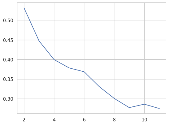
Silhouette score

Compute the mean Silhouette Coefficient of all samples. See scikit-learn documentation for details.

cgram.silhouette_score()

2     0.531540
3     0.447219
4     0.399584
5     0.378367
6     0.368591
7     0.330913
8     0.300624
9     0.277248
10    0.285975
11    0.274908
Name: silhouette_score, dtype: float64

Once computed, resulting Series is available as cgram.silhouette_. Calling the original method will recompute the score.

cgram.silhouette_.plot();

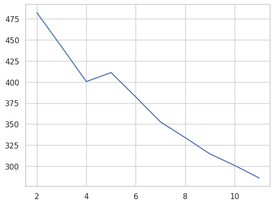
Calinski and Harabasz score

Compute the Calinski and Harabasz score, also known as the Variance Ratio Criterion. See scikit-learn documentation for details.

cgram.calinski_harabasz_score()

2     482.191469
3     441.677075
4     400.410025
5     411.158668
6     382.302322
7     352.552704
8     333.912576
9     314.589318
10    300.899582
11    285.934254
Name: calinski_harabasz_score, dtype: float64

Once computed, resulting Series is available as cgram.calinski_harabasz_. Calling the original method will recompute the score.

cgram.calinski_harabasz_.plot();

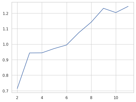
Davies-Bouldin score

Compute the Davies-Bouldin score. See scikit-learn documentation for details.

cgram.davies_bouldin_score()

2     0.714064
3     0.943553
4     0.944215
5     0.971900
6     0.994783
7     1.074578
8     1.141701
9     1.231220
10    1.203771
11    1.243758
Name: davies_bouldin_score, dtype: float64

Once computed, resulting Series is available as cgram.davies_bouldin_. Calling the original method will recompute the score.

cgram.davies_bouldin_.plot();

Acessing labels

Clustergram stores resulting labels for each of the tested options, which can be accessed as:

cgram.labels_

	1	2	3	4	5	6	7	8	9	10	11
0	0	1	2	1	2	2	1	6	1	3	2
1	0	1	2	1	2	2	1	2	5	6	2
2	0	1	2	1	2	2	1	2	5	6	9
3	0	1	2	1	2	2	1	6	1	3	9
4	0	1	2	1	0	0	3	6	1	2	1
...	...	...	...	...	...	...	...	...	...	...	...
337	0	0	1	0	3	1	6	4	0	4	4
338	0	0	1	0	3	1	6	4	0	4	4
339	0	0	1	2	1	4	5	5	3	8	8
340	0	0	1	0	3	1	2	1	6	0	0
341	0	0	1	2	1	4	2	1	6	0	0

342 rows × 11 columns

Saving clustergram

If you want to save your computed clustergram.Clustergram object to a disk, you can use pickle library:

import pickle

with open('clustergram.pickle','wb') as f:
    pickle.dump(cgram, f)

with open('clustergram.pickle','rb') as f:
    loaded = pickle.load(f)